Table of Contents
Open Table of Contents
Preface
- 相关书籍
- 学者博客
- Important Packages
- Summary Models: modelsummary, gtsummary
- Plot Results: sjPlot
The question isn’t whether you’ve omitted anything, it’s how important the omission is.
Your last line of defense is your gut. 如果你在直觉上感觉都有些不对劲,那大概率是错的。
- Begin with a question, a GOOD question
- 这个问题是可以回答的,最好是可以通过数据获得答案
- 这个问题的答案,有助于我们理解世界运行的规律,也就是具有理论性
- 我对这个问题的可能结果,有着初步的认识,感性的、理论的认识
- 这个问题是可行的,我有能力去收集数据,数据的来源是可靠、准确的
- 我为了检验答案所设计的研究是合理的
- 尽量让问题简单化
- Describe variables:当一个数据左偏或者右偏时,可以使用 log 让其变正态
- Identification:Find Data Generating Process. That process - finding where the variation you’re interested in is lurking and isolating just that part so you know that you’re answering your research question - is called identification.
- Using theory, paint the most accurate picture possible of what the data generating process looks like
- Use that data generating process to figure out the reasons our data might look the way it does that don’t answer our research question
- Find ways to block out those alternate reasons and so dig out the variation we need
- Casual Diagrams:对于因果的识别,来源于既往的文献、理论以及现实经验。变量间的复杂关系会导致因果图趋于复杂,精简因果图:1. 去掉不重要的 2. 去掉冗余的 3. 去掉中介的,如果 A-B-C 的路径上,再没有别的变量影响,可以考虑精简为 A-C 4. 去掉无关的变量
- Front Doors and Back Doors:我们希望识别的效应都是从x出发走到y,这就是前门。然而,总有一些变量,他可能同时对 x 和 y 产生影响,m 到 x 的路径就是后门。控制变量的目的就是关闭后门,留下前门。
A. Regression
💡 寻找与主效应相关的变量,将他们都控制住
1. Error Terms / Residual
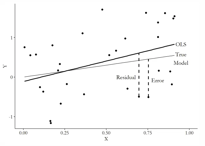
拟合模型中未知的部分就是Residual,未知的部分则是Error Error是由于模型的局限而导致的,Residual则还包括了样本的局限 由此,引出了外生性假设
假设1:外生性假设 Exogeneity Assumption If we want to say that our OLS estimates of will, on average, give us the population , then it must be the case that is uncorrelated with . 与 不相关,不意味着二者完全无关,这里的不相关只是指二者没有线性关系 与前面的研究设计部分相对应,外生性假设要求我们关闭因果图中的所有后门,仅留前门 换句话说,我们需要尽可能将那些影响较为直接的因素考虑在模型中 当 中与 直接具有线性关系时,通常会认为我们在模型中遗漏了一些重要变量 同时,我们遗漏一些东西是没事的——我们总会遗漏一些, 只要他与 无关就行
2. Hypothesis Testing
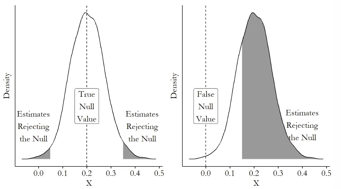
假设检验提供了一个捷径,我们通过拒绝 来告诉别人我的模型是对的 但是,不具有显著性的变量,不意味着他的估计就是错的,他只是在统计上不重要 不要通过修改数据来获得显著性 Never P-hacking 此外,显著性通过不意味着估计真实,如果标准误很大,那么研究结论很可能是一个侥幸 最后,显著性不是研究的全部,研究结论的重要与否更取决于你的故事
3. Variables
- 离散变量 Discrete Variable 虚拟变量,注意分类变量是与某一类别比,可用联合检验考察
library(car)
linearHypothesis(fit, hypothesis.matrix)- 多项式 Polynomials 通过观察 的散点图,如果需要多项式,那么图案应当具有规律性
- 变量转换 Variable Transformations 对 X 取对数:当变量有偏,尤其是右偏的时候可以通过取对数让分布正态 对 Y 取对数:让回归线性 取平方根:类似于取对数,与对数相比这个变换还能接受0 反双曲正弦变换 Inverse Hyperbolic: 可以接受0和负数 尾部处理 Winsorizing:专门用于处理异常值,将X%之后的值都替换为X%上的值 标准化 Standardizing:,目的是使模型易于解释
- 交互项 Interaction Terms X 对 Y 的影响: 一旦加入了交互项,单个系数可能会变得奇怪,需要将交互项都综合考虑进来
- 非线性回归 Nonlinear Regression 广义线性回归 Generalized Liner Models: 逻辑回归 Logit Link: 泊松回归 Probit Link:累积分布函数 使用 GLM 后,很难继续对系数进行更准确的描述,增加对需要通过边际效应求解 1. Marginal Effect at the Mean 取所有变量来 2. Average Marginal Effect
4. Standard Errors
假设2:正态假设 Normally Distributed The error term itself must be normally distributed. 不过这个假设不重要假设3:独立同分布 Independent and Identically Distributed The theoretical distribution of the error term is unrelated to the error terms of other observations and the other variables for the same observation (independent) as well as the same for each observation (identically distributed)
- 异方差下的标准误修正:Sandwich Estimator 和 Huber-White Standard Errors
library(tidyverse)

m1 <- causaldata::restaurant_inspections %>%
  lm(inspection_score ~ Year + Weekend, data = .) # 拟合

# 法1:使用AER包计算
library(AER); library(sandwich)
coeftest(m1, vcov = vcovHC(m1))
# 法2:也可以直接用modelsummary汇总出结果
library(modelsummary)
msummary(m1, vcov = 'robust',
		 stars = c('*' = .1, '**' = .05, '***' = .01))
# 法3:也可以用fixest直接进行回归分析
library(fixest)
feols(inspection_score ~ Year + Weekend, data = df, se = 'hetero')- 时间自相关下:Heteroskedasticity- and Autocorrelation-Consistent (HAC) Standard Errors、Newey-West estimator
library(tidyverse)

m2 <- causaldata::restaurant_inspections %>%
  group_by(Year) %>%
  summarize(Avg_Score = mean(inspection_score),
			Pct_Weekend = mean(Weekend)) %>%
  dplyr::filter(Year <= 2009) %>%
  lm(Avg_Score ~ Pct_Weekend, data = .) # 拟合

library(AER); library(sandwich)
coeftest(m2, vcov = NeweyWest)- Hierarchical Structure:clustered standard errors、Liang-Zeger standard errors
library(tidyverse)

m1 <- causaldata::restaurant_inspections %>%
  lm(inspection_score ~ Year + Weekend, data = .) # 拟合

# 法1
library(AER); library(sandwich)
coeftest(m1, vcov = vcovCL(m1, ~Weekend))
# 法2
library(modelsummary)
msummary(m1, vcov = ~Weekend,
		 stars = c('*' = .1, '**' = .05, '***' = .01))
# 法3
library(fixest)
feols(inspection_score ~ Year + Weekend,
	  cluster = ~ Weekend,
data = df)- 最后,Bootstrap,解决样本偏误问题的最完美的标准误
library(tidyverse); library(modelsummary); library(sandwich)

m1 <- causaldata::restaurant_inspections %>%
  lm(inspection_score ~ Year + Weekend, data = .) # 拟合

msummary(m1, vcov = function(x) vcovBS(x, R = 2000),
		 stars = c('*' = .1, '**' = .05, '***' = .01))
5. Additional Regression Concerns
- 样本权重 Sample Weights 当样本有偏时,可以通过调整权重来控制样本的分布
library(tidyverse); library(modelsummary)

df <- causaldata::restaurant_inspections %>%
  group_by(business_name) %>%
  summarize(Num_Inspections = n(),
			Avg_Score = mean(inspection_score),
			First_Year = min(Year))

# Add the weights argument to lm
m1 <- lm(Avg_Score ~ First_Year,
		 data = df,
		 weights = Num_Inspections)

msummary(m1, stars = c('*' = .1, '**' = .05, '***' = .01))

# 如果权重很复杂,可以 library(survey)- 共线性 Collinearity 一般情况下不会有完美的共线问题,但是当两个变量间 VIF 高于 0.9 时还是需要处理一下 VIF 高于 0.9 指的是 ,回归发现 大于 0.9
library(tidyverse)

m1 <- causaldata::restaurant_inspections %>%
  lm(inspection_score ~ Year, data = .) # 拟合

library(car)
vif(m1)- 测量误差 Measurement Error 经典测量误差可以不用处理 而当测量误差与自变量相关时,则需要进行处理
- 惩罚回归 Penalized Regression
library(tidyverse); library(modelsummary); library(glmnet)

# 数据处理
df <- causaldata::restaurant_inspections %>%
  select(-business_name)
X <- model.matrix(lm(inspection_score ~ (.)^2 - 1,
					 data = df))
numeric.var.names <- names(df)[2:3]
X <- cbind(X,as.matrix(df[,numeric.var.names]^2))
colnames(X)[8:9] <- paste(numeric.var.names,'squared')
Y <- as.matrix(df$inspection_score)
X <- scale(X); Y <- scale(Y)

# 找到一个最好的lambda,也就是cv.lasso$lambda.min
cv.lasso <- cv.glmnet(X, Y,
					  family = "gaussian",
					  nfolds = 20, alpha = 1)

# 运行真正的lasson模型
lasso.model <- glmnet(X, Y,
					  family = "gaussian",
					  alpha = 1,
					  lambda = cv.lasso$lambda.min)

# 查询那个变量被抛弃了,表现为-
lasso.model$beta
B. Matching
💡 找到一个除了主效应外,没有其他变化的样本
1. Weighted
匹配体现在数据表中,通过加权的方式来影响数据的生成与回归的结果
- 常见的匹配方式 One-to-One Matching, K-Nearest-Neighbor Matching, Radius Matching 一对一匹配将更多的引入偏差,半径匹配则将引入更多的方差 当控制组和对照组数量相当时,可以考虑使用一对一匹配,或者1对k匹配 当控制组数量远高于对照组时,可以考虑1对K匹配,或者半径匹配
- 计算匹配值的两种方式 Mahalanobis Distance: Propensity Score Matching
- 计算权重的两种方式 Kernel-based Weighting: Inverse Probability Weighting : 不过逆概率加权的方式,在处理接近0、1的概率时会出问题,需要进行处理 常见的方法是将倾向得分转化为优势比,然后再计算 P 计算半径的带宽,一般是匹配值的标准差,精确匹配的带宽则为0
2. Mahalanobis Distance Matching
基于 Mahalanobis Distance 的传统距离匹配
library(Matching); library(tidyverse)
br <- causaldata::black_politicians

# 被解释变量
Y <- br %>% pull(responded)
# 解释变量
D <- br %>% pull(leg_black)
# 用于匹配的变量
X <- br %>%
  select(medianhhincom, blackpercent, leg_democrat) %>%
  as.matrix()

# Weight = 2 指定使用 Mahalanobis distance
M <- Match(Y, D, X, Weight = 2, caliper = 1)
summary(M)

# 将匹配结果取出
matched_treated <- tibble(id = M$index.treated, weight = M$weights)
matched_control <- tibble(id = M$index.control, weight = M$weights)
matched_sets <- bind_rows(matched_treated, matched_control) %>%
  group_by(id) %>%
  summarize(weight = sum(weight))
# 与原始数据合并
matched_br <- br %>%
  mutate(id = row_number()) %>%
  left_join(matched_sets, by = 'id')

# 通过加权的方式加入到回归中
lm(responded ~ leg_black, data = matched_br, weights = weight)
3. Coarsened Exact Matching
Mahalanobis Distance 忽略了一些变量的作用,他会删除一些变量 如果我们假设所有的变量都很重要,就需要进行精确匹配 然而精确匹配要求距离为0,对于连续变量而言几乎不肯能有距离为0的变量 因此有必要先对变量进行粗化,将其作为类似类别的变量再进行匹配
library(cem); library(tidyverse)
br <- causaldata::black_politicians

# 取出需要用于匹配的变量,包括解释变量和被解释变量
brcem <- br %>%
  select(responded, leg_black, medianhhincom,
         blackpercent, leg_democrat) %>%
  na.omit() %>%
  as.data.frame() # Must be a data.frame, not a tibble

# 粗化变量
# 对于连续变量可以自动处理,但是二元变量需要手动处理

# 通过分位数来切割
# 这里数字为6,其实是分为了5类,去了中间的4个节点
inc_bins <- quantile(brcem$medianhhincom, (0:6)/6)

# 通过均匀分配来切割
create_even_breaks <- function(x, n) {
  minx <- min(x); maxx <- max(x)
  return(minx + ((0:n)/n)*(maxx-minx))}
# 与之前相同,6表示分为5类
bp_bins <- create_even_breaks(brcem$blackpercent, 6)
# 对于2维变量分为两类就行
ld_bins <- create_even_breaks(brcem$leg_democrat, 2)

# 记录区间
allbreaks <- list('medianhhincom' = inc_bins,
                  'blackpercent' = bp_bins,
                  'leg_democrat' = ld_bins)

# 匹配
c <- cem(treatment = 'leg_black', data = brcem,
         baseline.group =  '1',  # baseline.group 必须是对照组 treated group
         drop = 'responded',     # 被解释变量不应用于匹配
         cutpoints = allbreaks,
         keep.all = TRUE)

# 将匹配结果(权重)取出
brcem <- brcem %>%
  mutate(cem_weight = c$w)

# 回归
lm(responded~leg_black, data = brcem, weights = cem_weight) %>% summary()
# 也能用att
att(c, responded ~ leg_black, data = brcem)
# 论文中的回归结果
m1 <- lm(responded ~ leg_black*treat_out + nonblacknonwhite +
           black_medianhh + white_medianhh + statessquireindex +
           totalpop + urbanpercent, data = br, weights = cem_weight)
msummary(m1, stars = c('*' = .1, '**' = .05, '***' = .01))
4. Entropy Balancing
library(ebal); library(tidyverse); library(modelsummary)
br <- causaldata::black_politicians

# 被解释变量
Y <- br %>% pull(responded)
# 解释变量
D <- br %>% pull(leg_black)
# 匹配变量
X <- br %>%
  select(medianhhincom, blackpercent, leg_democrat) %>%
  # Add square terms to match variances if we like
  mutate(incsq = medianhhincom^2,
         bpsq = blackpercent^2) %>%
  as.matrix()

# 匹配
eb <- ebalance(D, X)

# 取出匹配结果
# Noting that this contains only control weights
br_treat <- br %>%
  filter(leg_black == 1) %>%
  mutate(weights = 1)
br_con <- br %>%
  filter(leg_black == 0) %>%
  mutate(weights = eb$w)
br <- bind_rows(br_treat, br_con)

m <- lm(responded ~ leg_black, data = br, weights = weights)
msummary(m, stars = c('*' = .1, '**' = .05, '***' = .01))
5. Propensity Score Matching
library(causalweight); library(tidyverse)
br <- causaldata::black_politicians

# We can estimate our own propensity score
m <- glm(leg_black ~ medianhhincom + blackpercent + leg_democrat,
         data = br, family = binomial(link = 'logit'))
# Get predicted values
br <- br %>%
    mutate(ps = predict(m, type = 'response'))
# "Trim" control observations outside of
# treated propensity score range
# (we'll discuss this later in Common Support)
minps <- br %>%
    filter(leg_black == 1) %>%
    pull(ps) %>%
    min(na.rm = TRUE)
maxps <- br %>%
    filter(leg_black == 1) %>%
    pull(ps) %>%
    max(na.rm = TRUE)
br <- br %>%
    filter(ps >= minps & ps <= maxps)

# Create IPW weights
br <- br %>%
    mutate(ipw = case_when(
    leg_black == 1 ~ 1/ps,
    leg_black == 0 ~ 1/(1-ps)))

# And use to weight regressions (The standard errors will be wrong
# here unless we bootstrap the whole process - See the code examples
# from the doubly robust estimation section or the simulation chapter)
lm(responded ~ leg_black, data = br, weights = ipw)

# Or we can use the causalweight package!
# First, pull out our variables
# Outcome
Y <- br %>%
    pull(responded)
# Treatment
D <- br %>%
    pull(leg_black)
# Matching variables
X <- br %>%
    select(medianhhincom, blackpercent, leg_democrat) %>%
    as.matrix()

# Note by default this produces average treatment effect,
# not average treatment on the treated, and trims propensity
# scores based on extreme values rather than matching treated range
IPW <- treatweight(Y, D, X, trim = .001, logit = TRUE)

# Estimate and SE
IPW$effect
IPW$se
6. Estimation with Matched Data
# 检验面板平衡
library(Matching)
MatchBalance(Y ~ D + X)

library(boot); library(tidyverse)
br <- causaldata::black_politicians

# Function to do IPW estimation with regression adjustment
ipwra <- function(br, index = 1:nrow(br)) {
  # Apply bootstrap index
  br <- br %>% slice(index)

  # estimate and predict propensity score
  m <- glm(leg_black ~ medianhhincom + blackpercent + leg_democrat,
           data = br, family = binomial(link = 'logit'))
  br <- br %>%
    mutate(ps = predict(m, type = 'response'))

  # Trim control observations outside of treated PS range
  minps <- br %>%
    filter(leg_black == 1) %>%
    pull(ps) %>%
    min(na.rm = TRUE)
  maxps <- br %>%
    filter(leg_black == 1) %>%
    pull(ps) %>%
    max(na.rm = TRUE)
  br <- br %>%
    filter(ps >= minps & ps <= maxps)

  # Create IPW weights
  br <- br %>%
    mutate(ipw = case_when(
      leg_black == 1 ~ 1/ps,
      leg_black == 0 ~ 1/(1-ps)))

  # Estimate difference
  w_means <- br %>%
    group_by(leg_black) %>%
    summarize(m = weighted.mean(responded, w = ipw)) %>%
    arrange(leg_black)

  return(w_means$m[2] - w_means$m[1])
}

b <- boot(br, ipwra, R = 200)
# See estimate and standard error
b
C. Simulation
1. Why We Simulate
测试估计在特定的样本中是否会有真正的效果,进而了解估计的抽样分布
同时,可以看到估计对某些假设的敏感性。验证某一假设不成立时,估计的有效性
library(tidyverse)
set.seed(1000)

# We must pick a number of observations, here 200
d <- tibble(eps = rnorm(200), # by default mean 0, sd 1
    Y = runif(200), # by default from 0 to 1
    X = sample(0:1, # sample from values 0 and 1
               200, # get 200 observations
               replace = TRUE, # sample with replacement
               prob = c(.8, .2))) # Be 1 20% of the time
2. Coding
创建数据
library(tidyverse)
library(purrr)
set.seed(1000)

# N for number of individuals, T for time periods
create_clus_data <- function(N = 200, T = 10) {
    # We're going to create errors clustered at the ID level.
    panel_data <- crossing(ID = 1:N, t = 1:T) %>%
        # Individual/time-varying data
        mutate(W = runif(n(), 0, .1))

    # Now an individual-specific error cluster
    indiv_data <- tibble(ID = 1:N,
                         C = rnorm(N))

    # Join them
    panel_data <- panel_data %>%
        full_join(indiv_data, by = 'ID') %>%
        # Create X, caused by W1 and W2
        mutate(X = 2*W + rnorm(n())) %>%
        # The error term has two components: the individual
        # cluster C, and the individual-and-time-varying element
        mutate(Y = 3*X + (C + rnorm(n())))

    return(panel_data)
}

create_clus_data(100,5)

# A function for estimation
est_model <- function(N, T) {
  # Get our data. This uses create_clus_data from earlier
  d <- create_clus_data(N, T)

  # Run a model that should be unbiased
  # if clustered errors themselves don't bias us!
  m <- lm(Y ~ X + W, data = d)

  # Get the efficient on X, which SHOULD be true value 3 on average
  x_coef <- coef(m)['X']

  return(x_coef)
}

# Run our model
est_model(200, 5)

# Estimate our model 1000 times (from 1 to 1000)
estimates <- 1:1000 %>%
  # Run the est_model function each time
  map_dbl(function(x) est_model(N = 200, T = 5))
3. Power Analysis
library(tidyverse); library(purrr); library(broom)
set.seed(1000)

# Follow the description in the text for data creation. Since we want
# to get minimum sample size and minimum detectable effect, allow both
# sample size and effect to vary.
# diff is the difference in effects between boys and girls
create_data <- function(N, effect, diff) {
    d <- tibble(W = rnorm(N),
        girl = sample(0:1, N, replace = TRUE)) %>%
        # A one-SD change in W makes treatment 10% less likely
        mutate(Training = runif(N) + .1*W < .5) %>%
        mutate(Test = effect*Training + diff*girl*Training +
                      4*W + rnorm(N, sd = 9))

    return(d)
}

# Our estimation function
est_model <- function(N, effect, diff) {
    d <- create_data(N, effect, diff)

    # Our model
    m <- lm(Test~girl*Training + W, data = d)
    tidied <- tidy(m)

    # By looking we can spot that the interaction
    # term is in the 5th row
    sig <- tidied$p.value[5] < .05

    return(sig)
}

# Iteration function!
iterate <- function(N, effect, diff, iters) {
    results <-  1:iters %>%
    map_dbl(function(x) {
        # To keep track of progress
        if (x %% 100 == 0) {print(x)}

        # Run our model and return the result
        return(est_model(N, effect, diff))
    })

    # We want to know statistical power,
    # i.e., the proportion of significant results
    return(mean(results))
}

# Let's find the minimum sample size
mss <- tibble(N = c(10000, 15000, 20000, 25000))
mss$power <- c(10000, 15000, 20000, 25000) %>%
    # Before we had to do function(x) here, but now the argument we're
    # passing is the first argument of iterate() so we don't need it
    map_dbl(iterate, effect = 2, diff = .8, iter = 500)
# Look for the first N with power above 90%
mss

# Now for the minimum detectable effect
mde <- tibble(effect = c(.8, 1.6, 2.4, 3.2))
mde$power <-  c(.8, 1.6, 2.4, 3.2) %>%
    map_dbl(function(x) iterate(N = 2000, effect = 2,
      diff = x, iter = 500))
# Look for the first effect wth power above 90%
mde
4. Bootstrap
library(tidyverse); library(boot)
set.seed(1000)

# Get our data set
data(mtcars)

# Our estimation function. The first argument must be the data
# and the second the indices defining the bootstrap sample
est_model <- function(d, index) {
    # Run our model
    # Use index to pick the bootstrap sample
    m <- lm(hp ~ mpg + wt, data = d[index,])

    # Return the estimate(s) we want to bootstrap
    return(c(coef(m)['mpg'],
             coef(m)['wt']))
}

# Now the bootstrap call!
results <- boot(mtcars,    # data
                est_model, # Estimation function,
                1000)      # Number of bootstrap simulations

# See the coefficient estimates and their bootstrap standard errors
results
Others
# T test
library(tidyverse)
(t.t.df <- data.frame(data$group, data$x1, data$x2) %>%
    select_if(is.numeric) %>%
    map_df(~ broom::tidy(t.test(. ~ data$group))))
1. Structural Equation
# set relevant data into new data frame
SR <- data1[,54:56];
# alpha and omega test
alpha(SR); omega(SR)
# test validity
KMO(SR); cortest.bartlett(SR)
2. Path Analysis
"Path Analysis"
# use likelihood = "wishart" to make result similar to AMOS
# use se = "bootstrap" in sem function if needed
model <- "# define structure
          PBb ~ b1 * SI + b2 * SC + c1 * MH + c2 * FM + c3 * SR +
                c4 * ew + c5 * PltStatus + c6 * Mar + pc + cb +
                Gender + Age + Punishment + Location
          SI ~ a11 * MH + a12 * FM + a13 * SR + Gender + Age
          SC ~ a21 * ew + a22 * PltStatus + a23 * Mar + Gender + Age

          # define indirect pathway
          # MH-SI-PB
          indirect1 := a11 * b1
          # FM-SI-PB
          indirect2 := a12 * b1
          # SR-SI-PB
          indirect3 := a13 * b1
          # ew-SC-PB
          indirect4 := a21 * b2
          # PltStatus-SC-PB
          indirect5 := a22 * b2
          # Mar-SC-PB
          indirect6 := a23 * b2
          # difference between SC and SI
          contrast := indirect1 + indirect2 + indirect3 -
                      indirect4 - indirect5 - indirect6
          total := c1 + c2 + c3 + c4 + (a11*b1) + (a12*b1) + (a13*b1) +
                  (a21*b2) + (a22*b2) + (a23*b2)
"; fit.pa <- sem(model, data = data1, likelihood = "wishart", se = "bootstrap")
summary(fit.pa, fit = T, rsquare = T)